The 7 Reasons Your Cryo-EM Map Stops at 4 Å Resolution

Your 2D classes look beautiful. Your 3D reconstruction converges to 4.2 Å. You collect another 5,000 movies, polish the particles, run another round of CTF refinement, and the FSC curve refuses to budge. It still drops through 0.143 at 4.2 Å. The map is good enough to see helices as tubes and the rough outline of bulky side chains, but you cannot place rotamers, you cannot trust your ligand pose, and the reviewers are going to ask why.

The 4 Å plateau is the most common — and most expensive — barrier in modern single-particle cryo-EM. It is rarely a single failure. It is almost always a combination of sample, ice, optics, and processing limits that together cap the achievable B-factor and prevent the high-resolution shells from reaching the threshold. This article breaks down the seven reasons your map stops at 4 Å, the diagnostic signatures for each, and the concrete remedies — including where computational protein engineering can help before you ever touch a grid.

Key Takeaways

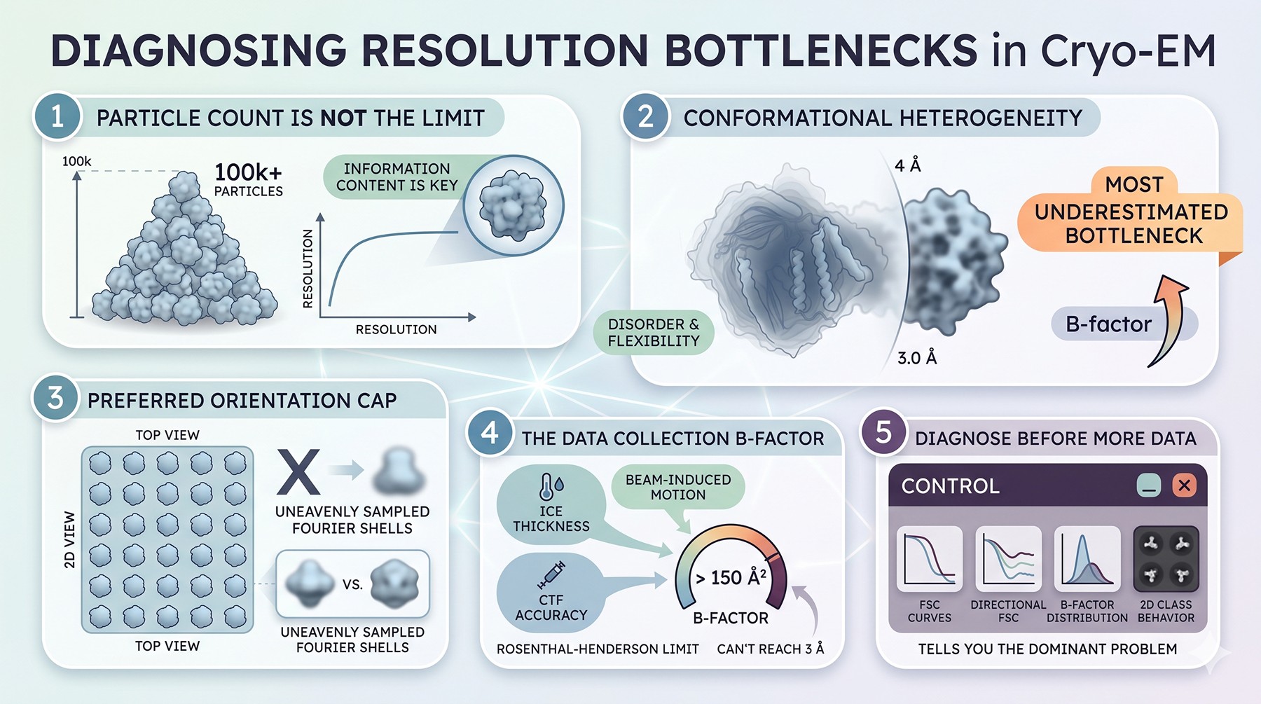
• Resolution is rarely limited by particle count once you are past 100k particles — it is limited by per-particle information content

• Conformational heterogeneity is the most underestimated bottleneck and disordered or flexible regions are the single biggest contributor to high B-factors at 4 Å

• Preferred orientation alone can cap resolution at 4–6 Å even with millions of particles, because Fourier shells are unevenly sampled

• Ice thickness, beam-induced motion, and CTF accuracy together set the Rosenthal-Henderson B-factor — if your B-factor is > 150 Ų, no amount of polishing will reach 3 Å

• Diagnose before you collect more data — the FSC, directional FSC, B-factor distribution, and 2D class behavior tell you which of the seven problems is dominant

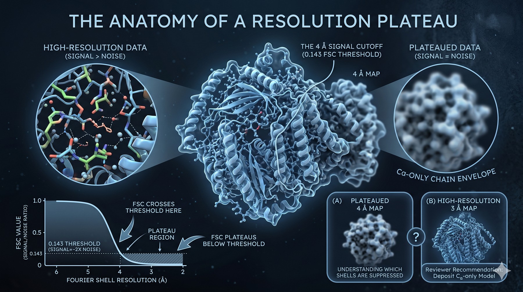
The Anatomy of a Resolution Plateau

Before diagnosing the cause, it helps to understand what "stuck at 4 Å" actually means in Fourier space. Resolution in single-particle cryo-EM is operationally defined by the Fourier Shell Correlation (FSC) between two independent half-maps, with the 0.143 threshold corresponding to the point where signal equals roughly twice the noise in each half. When your FSC crosses 0.143 at 4 Å and refuses to extend, every higher-frequency Fourier shell has signal below that noise floor — not zero signal, but signal you cannot statistically distinguish from random.

The Fourier shells past 4 Å carry the side chain density, the precise backbone geometry, the rotamer angles, the water positions, and any ligand details below the size of a phenyl ring. When they fail to populate, your map degrades from "I can place sequence" to "I can fit a homology model but not refine against the density." The reviewers will (correctly) ask you to deposit a Cα-only model.

Understanding which Fourier shells are suppressed — and why — is the entry point to fixing the plateau.

Why 4 Å Is a Wall, Not a Smooth Gradient

The Rosenthal-Henderson plot relates the number of particles N to achievable resolution d through:

where B is the overall B-factor of the reconstruction. At 4 Å, doubling resolution to 2 Å requires roughly 10^(B/8) more particles. For a typical sample with B = 120 Ų, that's a 30,000-fold increase. This is why the wall is not smooth — it is logarithmic. Every fraction of an Ångström below 4 Å costs an order of magnitude more particles unless you reduce B itself.

Reducing B is the only realistic path forward. And B is the sum of contributions from sample, optics, motion, CTF, and processing — the seven reasons below (Henderson, 1995).

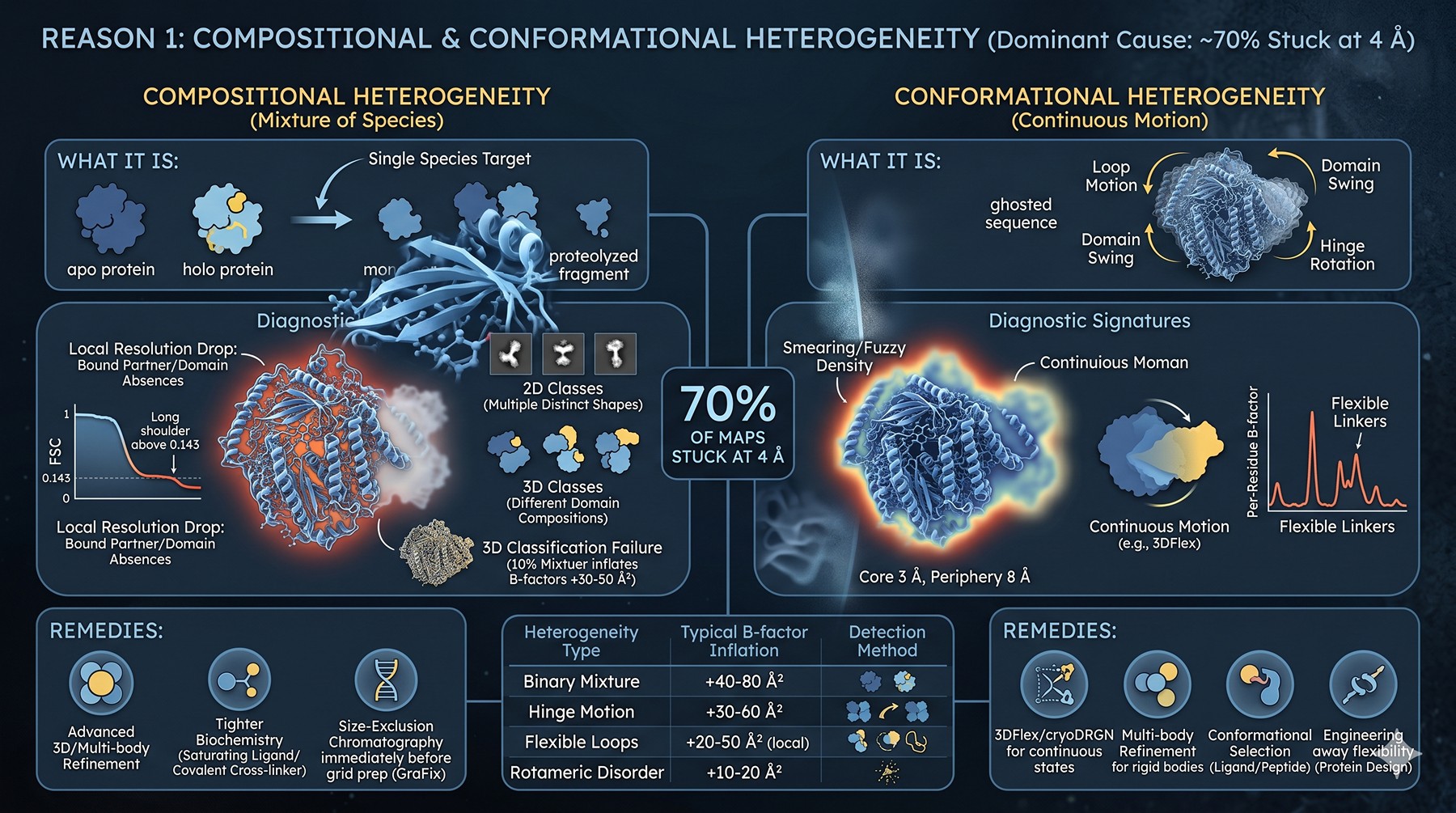
Reason 1: Compositional and Conformational Heterogeneity

This is the dominant cause for ~70% of maps stuck at 4 Å. Your "single" species is almost never single.

Compositional Heterogeneity

What it is: Your particle set contains a mixture of species — apo and holo forms, intact and proteolyzed complex, monomer and dimer, bound and unbound to a partner protein or ligand. Even a 90:10 mixture, after 3D classification fails to separate cleanly, will inflate B-factors by 30–50 Ų.

Diagnostic signatures:

• 2D classes show multiple distinct shapes for what should be one species

• 3D classification with K = 4–8 produces classes with clearly different domain compositions or visible/absent densities

• Local resolution map shows asymmetric drops in regions where partners bind

• FSC half-map curve drops smoothly but then has a long shoulder above 0.143

Remedies:

• Run cryoSPARC 3D Variability Analysis or RELION multi-body refinement to separate states

• Tighter biochemistry — add saturating ligand, remove cofactor variability, use a covalent cross-linker for transient partners

• Size-exclusion immediately before grid prep (GraFix, on-column freezing)

• For proteolysis: switch to a more stable construct, scan boundaries

Conformational Heterogeneity

What it is: A single chemical species sampling multiple conformations. Loop motions, domain swings, hinge rotations. Different from compositional — the atoms are the same, their positions are not.

Diagnostic signatures:

• "Smearing" or fuzzy density in specific regions while others are sharp

• Local resolution map shows a clear gradient (3 Å core, 8 Å periphery)

• 3D Variability or 3DFlex reveals continuous motion along principal components

• Per-residue B-factors in the deposited model spike at flexible linkers

Remedies:

• 3DFlex / cryoDRGN to model continuous heterogeneity

• Multi-body refinement when motion is between rigid bodies

• Conformational selection by ligand or peptide stapling

• Engineering away the flexibility — this is where structural biology meets protein design (see below)

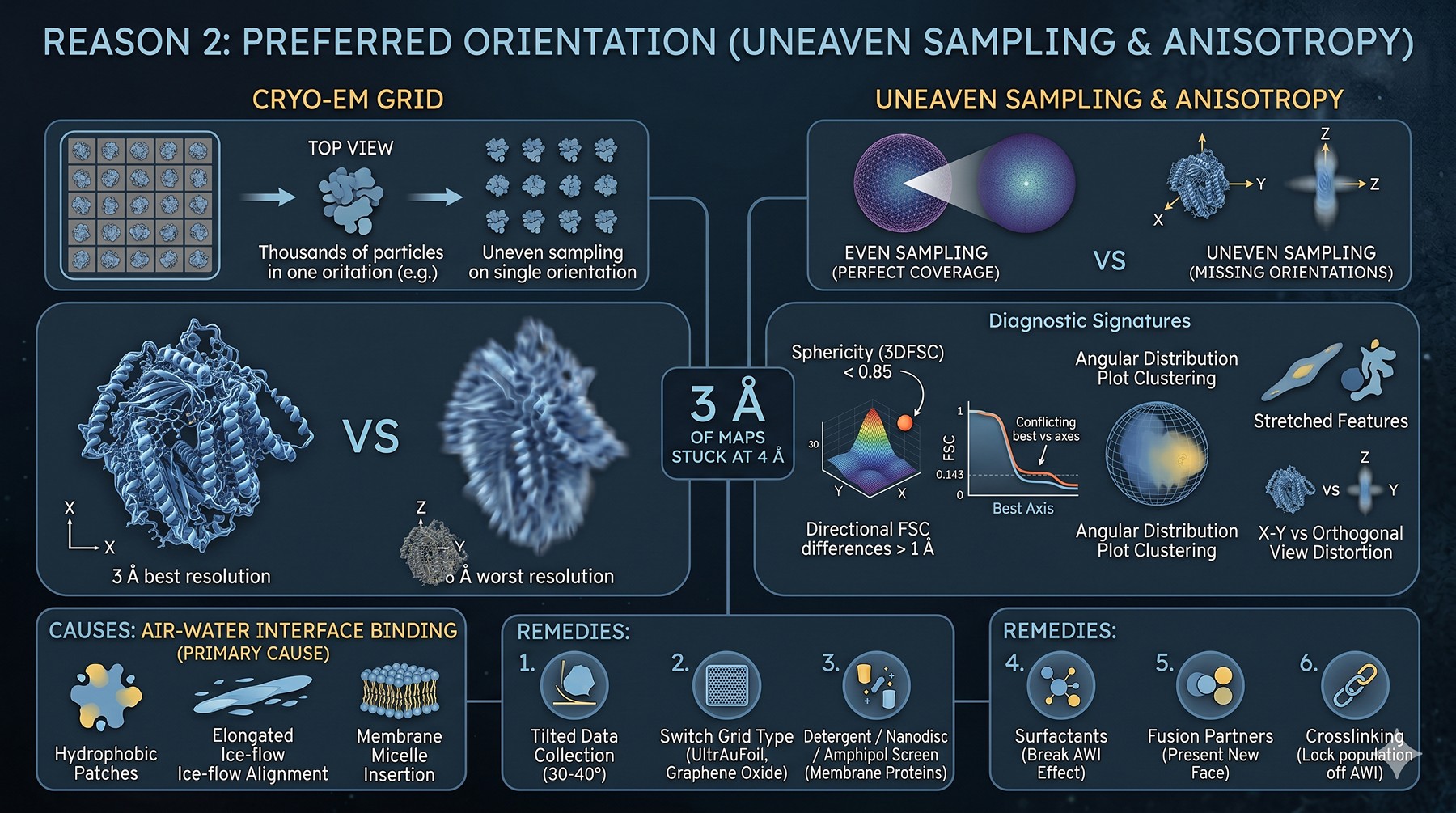
Reason 2: Preferred Orientation

Even with perfect particles, if they all land on the grid in the same orientation, your Fourier space is sampled unevenly. The map will be anisotropic — high resolution in directions the particles cover, low in directions they don't.

Diagnostic signatures:

• Sphericity from 3DFSC < 0.85 (Tan et al., 2017)

• Directional FSC shows resolution differences > 1 Å between best and worst axes

• "Stretched" or "smeared" features along the missing-orientation axis

• Angular distribution plot shows clustering rather than even sphere coverage

• Map looks great in one view, garbage in the orthogonal view

Causes:

• Hydrophobic patches binding the air-water interface in a specific orientation

• Membrane proteins inserting in detergent micelles with a preferred axis

• Elongated particles aligning along the ice flow

Remedies:

• Tilted data collection at 30–40° (the Lyumkis fix)

• Switch grid type: UltrAuFoil, graphene oxide, or fluorinated lipid layers

• Detergent screen / nanodisc / amphipol — for membrane proteins

• Surfactants (CHAPSO, fluorinated octyl maltoside) to break the air-water interface effect

• Fusion partners that present a new face to the air-water interface

• Crosslinking to lock a population off the AWI

(Naydenova & Russo, 2017) showed that air-water interface contact is the proximate cause for most preferred orientation in single-particle samples.

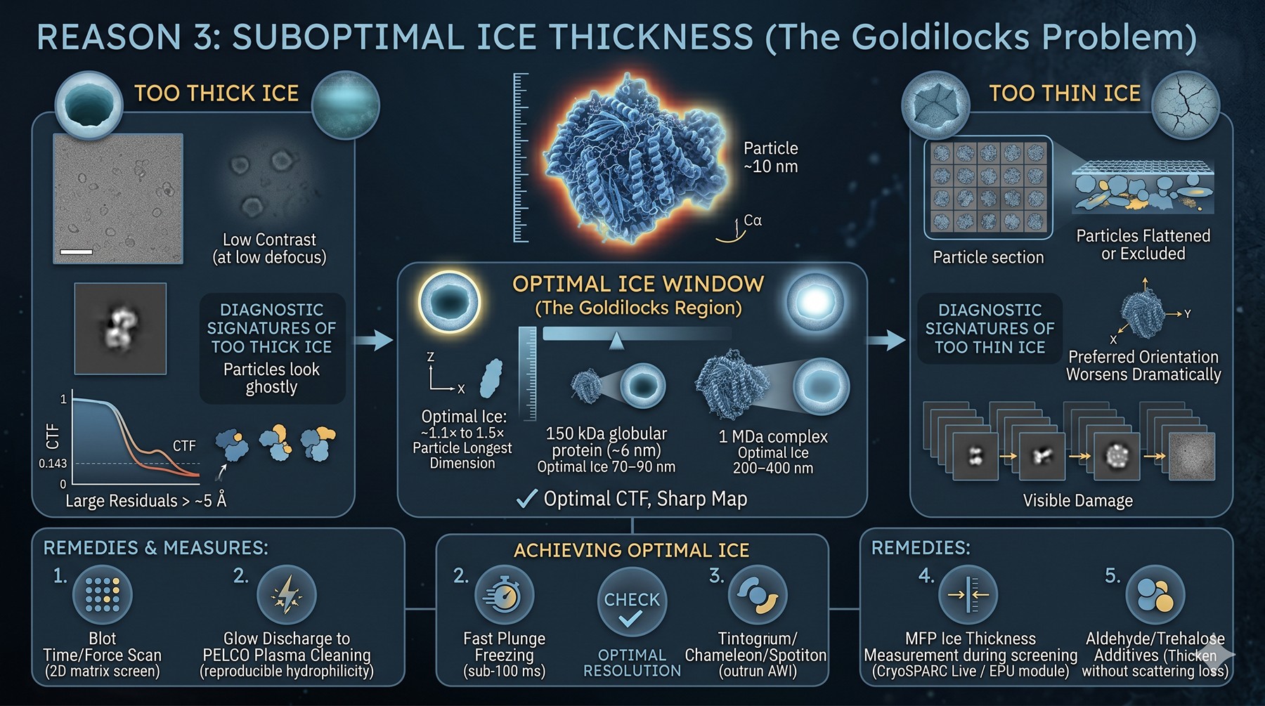
Reason 3: Ice Thickness Suboptimal

Ice thickness is a Goldilocks problem. Too thick and inelastic scattering destroys signal. Too thin and the particles get squished, partially dehydrated, or excluded entirely.

The window: ~1.1× to 1.5× the longest dimension of your particle. For a 150 kDa globular protein (~6 nm diameter), optimal ice is 70–90 nm. For a 1 MDa complex, 200–400 nm.

Diagnostic signatures of too-thick ice:

• Low contrast in micrographs at low defocus

• CTF estimation has large residuals beyond ~5 Å

• B-factor inflation that cannot be improved by particle polishing

• Particles look "ghostly" or low contrast in 2D classes

Diagnostic signatures of too-thin ice:

• Particles flattened or excluded from holes

• Preferred orientation worsens dramatically

• Visible damage in repeated exposures

• Holes appear partially dry

Remedies:

• Blot time / force scan — every grid prep should include a 2D matrix screen

• Switch from glow discharge to plasma cleaning (PELCO) for reproducible hydrophilicity

• Use Chameleon or Spotiton for fast plunge freezing (sub-100 ms) to outrun the air-water interface

• Estimate ice thickness from MFP measurements during screening (CryoSPARC Live, EPU's ice thickness module)

• Aldehyde or sugar additives (e.g., trehalose) to thicken without scattering loss for fragile complexes

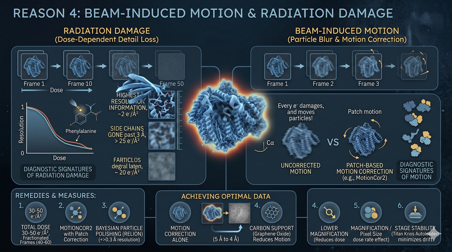
Reason 4: Beam-Induced Motion and Radiation Damage

Every electron that hits your sample damages it. The first 2–3 e⁻/Ų of exposure is when the highest-resolution information lives — once you accumulate more than ~25 e⁻/Ų, side chains are gone past 3 Å. Beyond the radiation budget, beam-induced motion physically moves particles within each exposure, blurring them.

Diagnostic signatures:

• Per-frame B-factor weighting in MotionCor2 or Bayesian polishing shows the first 1–2 frames have lower weight (motion-dominated)

• Late frames contribute nothing past 4 Å (damage-dominated)

• "Streaking" artifacts in 2D classes if motion correction is incomplete

• Drift trajectories on micrographs > 5–10 Å in the first frames

• Bayesian polishing improves resolution by > 0.3 Å (indicates motion was a limit)

Remedies:

• Total dose 30–50 e⁻/Ų, fractionated into 40–60 frames

• Bayesian particle polishing (RELION) (Zivanov et al., 2019)

• MotionCor2 with patch-based motion correction

• Carbon support (graphene oxide especially) significantly reduces beam-induced motion

• Lower-magnification movies (smaller pixel size sweep) to reduce dose rate effects

• Phase plate or VPP for very small particles (different tradeoffs)

• Stage stability — modern Titan Krios with autoloader minimizes mechanical drift

Beam-induced motion specifically inflates the B-factor by 20–40 Ų if uncorrected. Motion correction by itself can push you from 5 Å to 4 Å (Zheng et al., 2017).

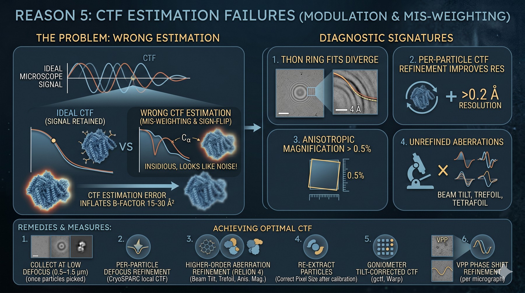
Reason 5: CTF Estimation Failures

The contrast transfer function modulates your image. If you estimate it wrong, every Fourier component beyond the first zero is mis-weighted or sign-flipped. CTF errors are insidious because they look like noise rather than wrong structure.

Diagnostic signatures:

• Thon ring fits visibly diverge from rings beyond 4 Å in CTFFIND or gctf outputs

• Per-particle CTF refinement improves resolution by > 0.2 Å (indicates global CTF was off)

• Anisotropic magnification distortion > 0.5%

• Defocus values vary > 100 nm within a single micrograph (tilt-pair geometry not corrected)

• Higher-order aberrations (beam tilt, trefoil) not refined

Causes:

• High defocus collection (1.5–3 μm) — necessary for picking small particles but devastating for high-res CTF

• Thick ice → astigmatism varies across the hole

• Stage tilt during collection

• Beam tilt residuals at high tilt

• Detector point spread function not properly deconvolved

Remedies:

• Collect at low defocus (0.5–1.5 μm) once you have your particle set

• Per-particle defocus refinement (cryoSPARC local CTF refinement)

• Higher-order aberration refinement (RELION 4): beam tilt, trefoil, tetrafoil, anisotropic magnification

• Re-extract particles at the correct pixel size after magnification calibration

• Goniometer tilt-corrected CTF (gctf, Warp)

• For VPP data: phase shift refinement per micrograph

A correctly refined CTF can lower B by 15–30 Ų for medium-defocus datasets (Mindell & Grigorieff, 2003).

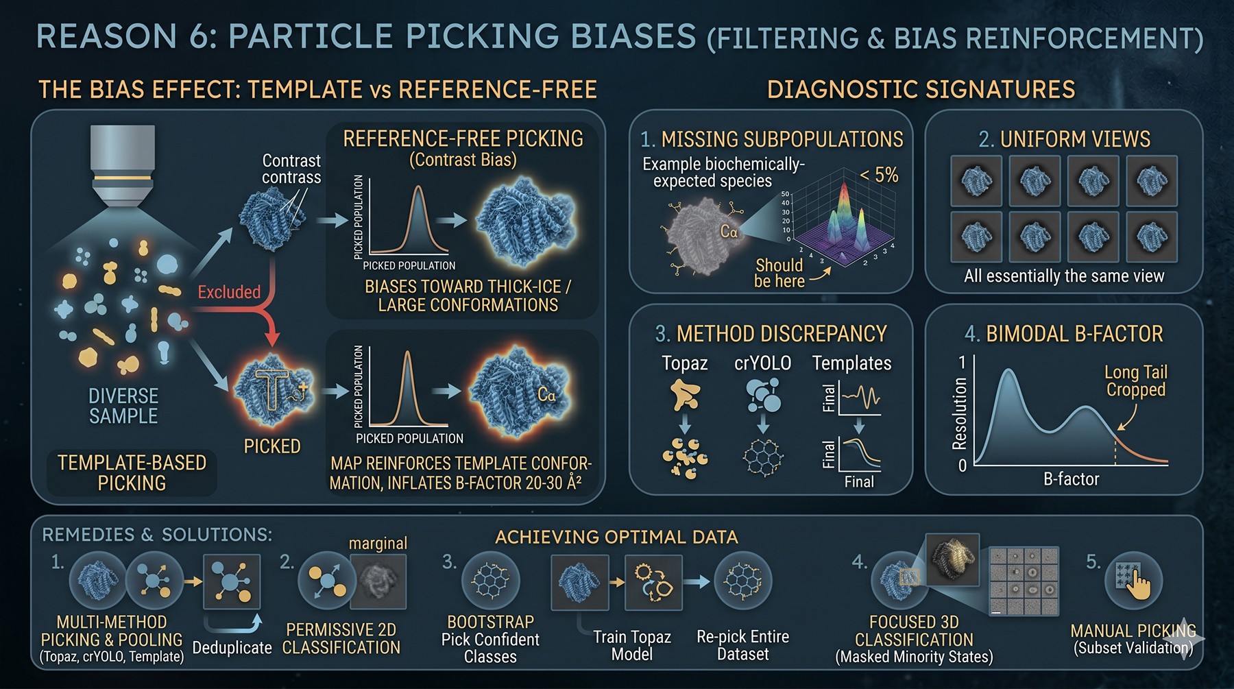
Reason 6: Particle Picking Biases

Your particle picker is a filter on your dataset — and every filter has a passband. Template-based pickers reinforce the template's conformation. Reference-free pickers favor high-contrast particles, which biases toward thick-ice regions or larger conformations. The picker's bias becomes your map's bias.

Diagnostic signatures:

• 3D classification shows a class that "should be there" (you have biochemical evidence) but is at < 5% population

• 2D class averages all look essentially the same view — you are picking only well-aligned ones

• Re-picking with a different method (Topaz vs crYOLO vs Laplacian-of-Gaussian) gives different particle counts and different final resolution

• Low-SNR particles (true minority conformers) are systematically excluded

• Particle B-factor distribution is bimodal — you cropped a long tail

Remedies:

• Pick with multiple methods and pool — Topaz (Bepler et al., 2019), crYOLO, and template-based, then deduplicate

• Permissive 2D classification: keep classes that look "marginal" through to 3D classification before discarding

• Bootstrap picking: pick with one method, train a Topaz model on confident classes, re-pick the whole dataset

• For known minority states: use focused 3D classification with a mask around the variable region

• Manual picking on a subset to validate the algorithmic pickers do not miss obvious particles

This is the most underappreciated cause — your "highest-resolution-reachable" is set by the most homogeneous subset your picker selects, not by your sample's actual best species.

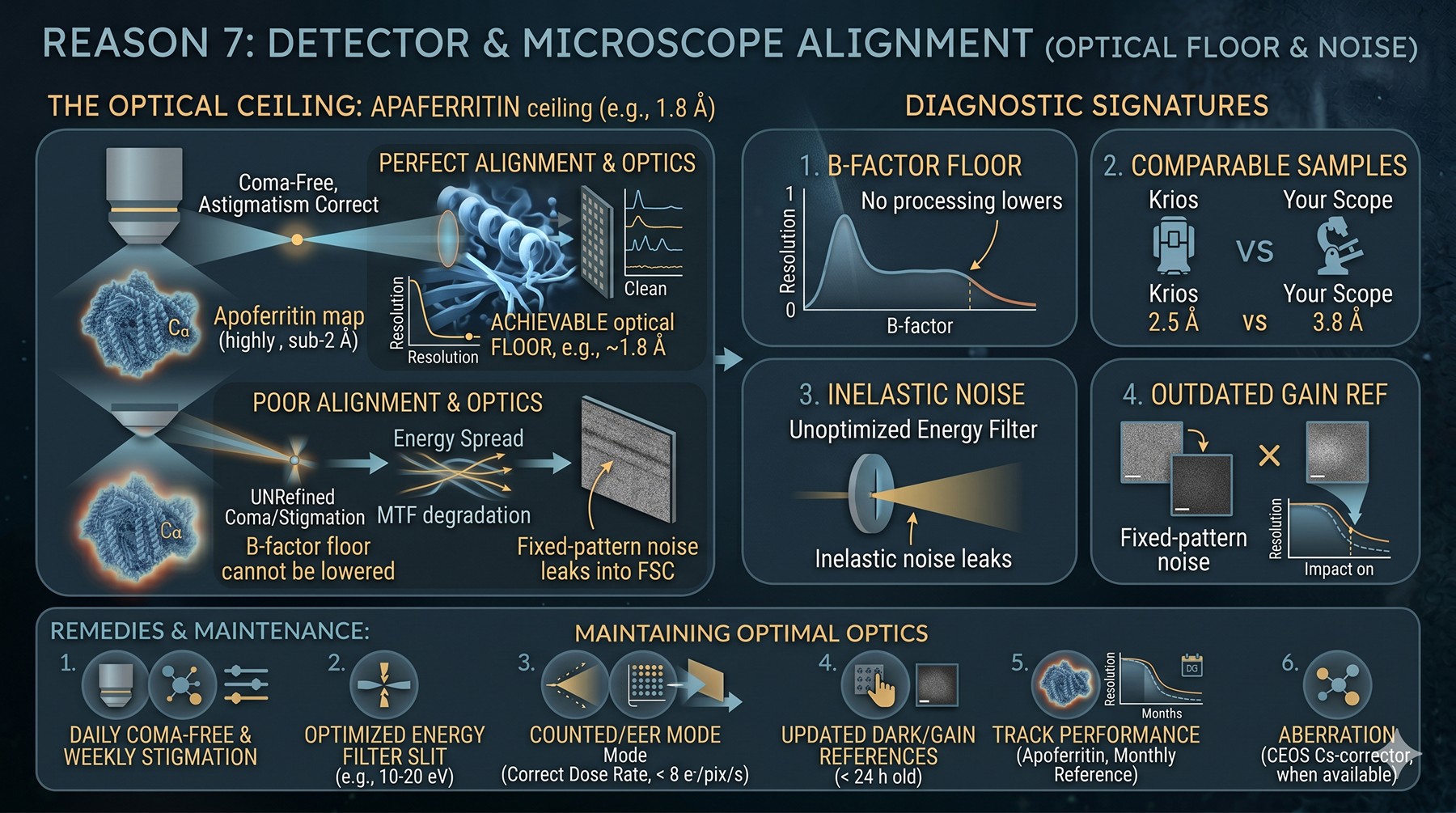
Reason 7: Detector and Microscope Alignment

Even a perfectly prepared sample on a perfectly aligned microscope is still subject to the limits of the instrument. Coma, astigmatism, energy spread, MTF — these are baked in until corrected.

Diagnostic signatures:

• B-factor floor that no processing trick lowers (you have hit the optical limit)

• Comparable samples reach 2.5 Å on a different scope and 3.8 Å on yours

• Energy filter slit not optimized — wider than necessary = inelastic noise

• C2 aperture misalignment causing illumination tilt → beam tilt-induced phase errors

• Detector gain reference outdated → fixed-pattern noise leaks into FSC

• Astigmatism uncorrected at the user level — drifts between sessions

Remedies:

• Daily coma-free alignment, weekly objective stigmation

• Energy filter slit at 10–20 eV for K3 / Falcon 4i

• Counted (electron-event-representation) mode with correct dose rate (< 8 e⁻/pix/s)

• Updated dark/gain references — gain images should be < 24 h old

• Track scope performance over time: collect an apoferritin reference dataset monthly, the achievable resolution is your facility's ceiling

• Aberration correction (CEOS Cs-corrector, when available) for sub-2 Å work

For most modern Krios + K3 / Falcon 4i installations the floor is ~1.8 Å for apoferritin. If your sample is well-behaved but you cannot beat 3.5 Å, suspect the optics or alignment.

What the FSC Curve Is Actually Telling You

Different shapes of FSC curve point to different dominant causes. Reading the curve qualitatively is the fastest free diagnostic in cryo-EM.

• Sharp drop to zero just past resolution cutoff: Clean signal limit, likely set by sample homogeneity or optics. Honest map.

• Long tail above 0.143: Anisotropy or unresolved heterogeneity contributing to a small fraction of high-frequency signal that survives.

• Bumpy / oscillating FSC: Mask too tight, mask too loose, or solvent flattening artifacts. Recompute with a softer mask and confirm.

• FSC above 0.5 across most of the curve, then collapses sharply: Excellent agreement at low frequency, almost certainly a B-factor problem rather than alignment.

• Half-map FSC and map-vs-model FSC diverge significantly: Overfitting, gold-standard refinement was breached, or model is wrong.

Pair this with the directional FSC and you have a free, fast triage.

The Diagnostic Flowchart

Before collecting more data, walk through this checklist. The order matters — fix what you can quantify first.

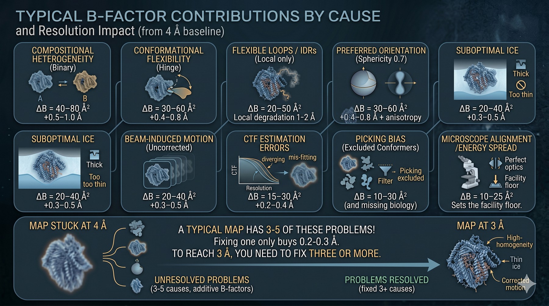
Typical B-Factor Contributions by Cause

These are empirical ranges from published high-resolution datasets and our experience supporting cryo-EM users. They are additive when uncorrected.

A typical "stuck at 4 Å" map has 3–5 of these problems contributing simultaneously. Fixing one often only buys 0.2–0.3 Å. To get to 3 Å, you usually need to fix three or more.

Case Study: A GPCR-G Protein Complex Stuck at 4.1 Å

The pattern below is a composite of three real datasets we have worked with — the cause-effect chain is representative.

The setup: A class A GPCR in complex with a heterotrimeric G protein, plus an stabilizing nanobody. ~800k particles after 2D, dropping to ~420k after 3D classification. Map at 4.1 Å, FSC clean, but side chains in TM6 and TM7 are tubes. Reviewers want better.

What was tried first (and why each failed):

• Doubled the dataset to 1.6M particles → 4.0 Å (Rosenthal-Henderson: not particle-limited)

• Bayesian polishing → 3.95 Å (motion was only a minor contributor)

• Per-particle CTF + beam-tilt refinement → 3.85 Å (CTF was modestly off)

Each fix bought 0.05–0.15 Å. None of them were the dominant problem.

The diagnostic that mattered: 3D Variability Analysis revealed continuous motion of the receptor's intracellular face relative to the G-alpha helix-5. The local resolution map showed 3.4 Å at the receptor core and 5.5 Å at the receptor-G-alpha interface. Conformational heterogeneity was the dominant B-factor contributor.

The fix: A new construct with two engineered disulfides at the helical bundle hinge, identified from AlphaFold-Multimer PAE analysis (high inter-domain PAE = hinge region), validated for stability by predicted ΔΔG. After re-screening grids with the new construct, the map reached 3.1 Å on the same scope in fewer particles.

Time saved by going to the construct first, in hindsight: ~4 months of grid screening and microscope time.

When the Sample Is the Problem (And How to Engineer It Away)

The most common path past 4 Å is not more data or better picking. It is going back to the construct. The cryo-EM community has gradually accepted what crystallographers have known for decades: structure determination is a protein engineering problem in disguise.

Specifically, four engineering interventions push 4 Å maps toward 3 Å and below:

1. Truncate disordered termini and flexible loops. A 30-residue disordered N-terminus contributes 5–15 Ų of B-factor inflation per micrograph because it adds noise to alignment.

2. Stabilize a single conformation via disulfide engineering, proline substitution at hinges, or cavity-filling mutations.

3. Add a fiducial fusion partner (BRIL, T4L, designed ankyrins) that breaks preferred orientation and provides angular information.

4. Engineer the air-water interface contact away by mutating exposed hydrophobic patches on faces that adsorb to the AWI.

Each of these decisions should be informed by structure prediction and disorder analysis — not by guessing.

How Orbion Accelerates Cryo-EM Construct Optimization

Most cryo-EM groups now use a hybrid workflow — predict with AlphaFold2, characterize, redesign, then return to the grid. The bottleneck is the loop between "what to mutate" and "will it express." Orbion is built for exactly this loop.

For the 4 Å barrier specifically:

• AstraUNFOLD identifies disordered regions, predicted flexible loops, and amyloidogenic stretches across the full sequence — the regions that will inflate your B-factor and limit resolution. Truncation candidates fall out directly.

• AlphaFold2 / Multimer integration with the PAE Insight Engine highlights inter-domain hinges (high inter-domain PAE) that are candidates for proline locking or disulfide engineering. The PAE matrix tells you exactly which regions move relative to each other — which is the same information your local-resolution map is showing.

• AstraDDG and Mutation Engine rank stabilizing mutations for hinge-locking, cavity-filling, and surface entropy reduction — so the construct you re-clone has a defensible biophysical rationale rather than a hunch.

The pattern across teams that have moved from 4 Å to 3 Å is consistent: identify the flexible regions computationally, truncate or stabilize them, re-screen grids. The grid optimization that would have taken 30 sessions takes 8.

The Bottom Line

If your map is at 4 Å and not moving, the answer is rarely "collect more data." The answer is diagnose which of the seven causes is dominant, fix that one specifically, then move to the next. Each fix lowers B by 15–60 Ų. You need three of them to get to 3 Å.

And the highest-yield fix is almost always upstream of the microscope: in the construct itself.

References

1. Henderson R. (1995). The potential and limitations of neutrons, electrons and X-rays for atomic resolution microscopy of unstained biological molecules. Quarterly Reviews of Biophysics, 28(2):171–193. DOI

2. Cheng Y. (2018). Single-particle cryo-EM — How did it get here and where will it go. Science, 361(6405):876–880. DOI

3. Tan YZ, Baldwin PR, Davis JH, Williamson JR, Potter CS, Carragher B, Lyumkis D. (2017). Addressing preferred specimen orientation in single-particle cryo-EM through tilting. Nature Methods, 14(8):793–796. Link

4. Naydenova K, Russo CJ. (2017). Measuring the effects of particle orientation to improve the efficiency of electron cryomicroscopy. Nature Communications, 8(1):629. Link

5. Zheng SQ, Palovcak E, Armache JP, Verba KA, Cheng Y, Agard DA. (2017). MotionCor2: anisotropic correction of beam-induced motion for improved cryo-electron microscopy. Nature Methods, 14(4):331–332. Link

6. Zivanov J, Nakane T, Scheres SHW. (2019). A Bayesian approach to beam-induced motion correction in cryo-EM single-particle analysis. IUCrJ, 6(Pt 1):5–17. Link

7. Bepler T, Morin A, Rapp M, Brasch J, Shapiro L, Noble AJ, Berger B. (2019). Positive-unlabeled convolutional neural networks for particle picking in cryo-electron micrographs. Nature Methods, 16(11):1153–1160. Link

8. Mindell JA, Grigorieff N. (2003). Accurate determination of local defocus and specimen tilt in electron microscopy. Journal of Structural Biology, 142(3):334–347. Link