1. Why this question matters
Finding new drugs is expensive. A typical compound costs about $2.6 billion and 10–15 years to bring to market, and most of that time is spent figuring out which molecules bind which proteins and how tightly. Machine learning has accelerated parts of this pipeline — AlphaFold, RoseTTAFold, and DiffDock have all moved the needle — but most ML models treat biology as a black box. They learn patterns from data without encoding the underlying physics.
Quantum computing offers a different route for molecular modeling. In principle, quantum hardware may represent electron behavior more naturally than classical methods, which could make some chemistry calculations more accurate or efficient over time. But the field is still approximation-heavy, and the real question is whether today’s near-term systems can deliver measurable value on practical drug discovery problems.
This blog walks through an end-to-end experiment: from downloading protein structures to training classifiers that predict binding sites.
2. Quantum biology — it’s real
Quantum mechanics is not something that appears only inside quantum computers. It already underlies ordinary biology.
Chemical bonds, light absorption, electron transfer, and molecular structure all depend on quantum physics. In that basic sense, biology is quantum from the ground up. The harder question is whether living systems make functional use of more delicate quantum effects, such as coherence, tunneling, or spin-dependent dynamics, in ways that matter for biology. In some cases, the answer appears to be yes, although the strength and biological relevance vary by system.
A few examples are especially important.
Photosynthesis. Spectroscopy experiments on photosynthetic complexes have shown coherence signatures during energy transfer. These results are real and important, but they should be described carefully: they do not mean plants are doing quantum computing. What they do suggest is that quantum-coherent effects can appear in biological energy transport on very short timescales.
Tunneling in biology. Protons and electrons can sometimes cross energy barriers through quantum tunneling rather than only by going over them classically. This has been implicated in parts of enzymatic catalysis and biological charge transfer, although the extent to which tunneling dominates depends on the specific system.
Magnetoreception. One of the leading explanations for how migratory birds sense Earth’s magnetic field is the radical-pair model, in which light triggers spin-dependent chemistry in cryptochrome proteins. This remains an active research area, but it is one of the strongest examples of a plausible biological sensing mechanism that depends on explicitly quantum spin dynamics.
For this post, though, I am interested in a more practical point.
When a small molecule binds to a protein, the interaction is ultimately governed by electrons: how charge redistributes, how orbitals interact, and how the local electronic environment changes. Classical force fields often approximate these effects very successfully, but some cases are harder than others, especially when binding depends on metal coordination, conjugated systems, charge transfer, or bond-making and bond-breaking. That is the real motivation here. Not the claim that biology is secretly a quantum computer, but the simpler idea that some biologically relevant interactions may benefit from more explicit quantum-informed features.
3. Why quantum might help drug discovery specifically
When a drug binds to a protein, the atoms are not just touching like Lego blocks.
What really matters is how the electrons in the drug and the protein respond to each other.
At a simple level, three things can happen:
-
The drug’s electron distribution shifts as it enters the binding pocket.
-
Charges can redistribute between nearby atoms, changing which interactions become stronger or weaker.
-
In some systems, especially those involving metals or aromatic rings, the interaction depends on more subtle electronic effects that are hard to capture with simple classical models.
Classical molecular dynamics is extremely useful and often works well. But many standard force fields approximate atoms with fixed or simplified charges and bonded interaction terms, which can miss important electronic effects. This becomes especially difficult when binding depends on effects such as polarization, charge transfer, dispersion, metal coordination, or bond formation and breaking.
This matters in several important cases:
-
Metal-binding enzymes
Active sites with zinc, iron, copper, or manganese are often hard to model because metals can have complicated coordination geometry, polarization, and partial charge-transfer behavior. Classical force fields often need special treatment here.
-
Cofactor binding
Molecules like heme, FAD, and NADH involve rich electronic structure, including conjugated systems and redox chemistry, which can be difficult to represent with simple fixed-charge models.
-
Covalent inhibitors
These drugs form a chemical bond with the target, so the problem is no longer just binding but also chemical reactivity. That usually requires quantum or QM/MM style treatment rather than ordinary classical MD alone. Covalent drugs are also a real and growing therapeutic class.
-
Halogen bonding
Bromine and iodine can form directional interactions driven by the so-called sigma hole, which is an electronic effect that classical models do not always capture well unless specially parameterized.
-
Pi stacking and aromatic interactions
These interactions are not just “flat rings sticking together.” They depend importantly on dispersion and other electronic effects, and quantum calculations are often used to understand them more accurately.
So the practical question is not whether all binding needs full quantum simulation.
It does not.
The more realistic question is: Can we capture the most important electronic effects in a compact form that machine learning can actually use?
4. The Variational Quantum Eigensolver (VQE)
VQE is the workhorse quantum algorithm for chemistry. It finds the ground state energy of a molecule — the lowest energy configuration of its electrons.
The physics: a molecule’s electrons obey the Schrödinger equation. The lowest eigenvalue of the molecular Hamiltonian H is the ground state energy. This is what determines binding strength, reaction rates, and all the properties we care about.
The math: finding the ground state of H is equivalent to solving
The classical approach — Full Configuration Interaction (FCI) — works on systems with ~20 electrons maximum. Any bigger and the number of configurations explodes.
The quantum approach — VQE — uses a parameterized quantum circuit to produce a trial state |ψ(θ)⟩, measures the energy ⟨ψ(θ)|H|ψ(θ)⟩ on a quantum computer, and classically optimizes the parameters θ to minimize that energy.
It’s a hybrid classical-quantum algorithm:
[Classical optimizer] ←→ [Quantum circuit evaluation]
        ↓                          ↓
  Update θ            Compute ⟨H⟩ for given θ
The quantum part is fast but noisy. The classical optimizer handles the search. This hybrid structure is why VQE works on noisy near-term hardware — no single circuit needs to be deep.
How we built the Hamiltonians
For each binding pocket fragment, we:
-
Placed the atoms in their experimentally determined positions (from PDB files)
-
Ran Hartree-Fock with PySCF to get the one-electron reference
-
Extracted molecular orbital integrals (h1 and h2)
-
Built the second-quantized Hamiltonian
-
Mapped it to qubits via Jordan-Wigner transformation
-
Simplified to 8 qubits by selecting a 4-electron, 4-orbital active space
The active space contains the chemically “interesting” orbitals — the HOMOs and LUMOs where most of the correlation lives. Core and virtual orbitals get frozen.
5. Our experimental pipeline
The experiment had eight stages, verified at each step:
-
Download 50 protein structures from the RCSB Protein Data Bank (RCSB)
-
Extract 32 binding pocket fragments covering 16 different ligand categories
-
Build molecular Hamiltonians for 26 light-atom fragments (metals deferred — they need larger basis sets)
-
Run VQE on 5 representative fragments with two different quantum circuits
-
Extract 10 quantum descriptors per binding category
-
Map descriptors to 220,471 residues from 1,000 BioLiP protein-ligand complexes
-
Train 4 classifiers on 3 different feature sets
-
Compare and decide whether quantum descriptors add value
The fragments we simulated
Five representative fragments covered diverse binding chemistry:
-
HEM (porphyrin) from PDB 4mqh — the iron-porphyrin cofactor in hemoglobin. 42 electrons, strong electron correlation from the iron d-orbitals.
-
AKG (organic acid) from PDB 1oij — alpha-ketoglutarate, a central metabolite in the Krebs cycle. 40 electrons.
-
CO3 (solvent) from PDB 1lfi — a carbonate ion. 46 electrons.
-
GDP (nucleotide) from PDB 5i4r — guanosine diphosphate, a purine nucleotide. 70 electrons.
-
G56 (other) from PDB 7con — a drug-like ligand with aromatic rings. 46 electrons.
Each fragment needed 8 qubits to simulate (4 electrons in 4 orbitals, with spin).
6. Physics-informed circuits: QNP vs HEA
The quantum circuit you choose matters enormously. We compared two:
Hardware-Efficient Ansatz (HEA). Generic layers of single-qubit rotations followed by CNOT entangling gates. Easy to implement, not tied to any physics. Often the “default” in quantum ML.
Qubit Number Preserving (QNP). A circuit structure from Anselmetti et al. (2021) that respects particle number conservation — a fundamental symmetry of chemistry. You can’t spontaneously create or destroy electrons, and the QNP circuit encodes that constraint. Uses the same gate as chemists have built into VQE ansätze for years, but applies them in a structured “fabric” across the qubits.
The difference is huge:
Left panel: QNP converges in about 20 iterations to its best answer. HEA takes 60+ iterations and uses vastly more parameters.
Right panel: On every single fragment, QNP used 6x fewer parameters and achieved 1.5-1.7x lower energy error. The numbers under each bar show the error ratio.
Why this matters for quantum ML broadly. The generic wisdom in deep learning is “more parameters, more expressivity, better results.” The quantum result is the opposite: encoding physical symmetries gives you a dramatically better inductive bias. A circuit that can only produce physically valid states finds the right answer faster than a circuit that can produce anything.
This lines up with recent theoretical work on “barren plateaus” — HEA circuits have exponentially vanishing gradients as you scale up, making them untrainable. Structured circuits like QNP avoid this.
7. The 10 quantum descriptors we extracted
For each binding category, we converted the converged VQE calculation into 10 numbers that summarize the quantum electronic structure:
| # | Descriptor | What it captures | Why it matters for binding |
|---|---|---|---|
| 1 | HOMO-LUMO gap | Energy gap between highest occupied and lowest unoccupied orbitals | Small gap = reactive, prone to electron transfer |
| 2 | Orbital entanglement entropy | Von Neumann-like entropy from natural occupations | High entropy = strong correlation, multi-reference character |
| 3 | Number of fractional orbitals | Orbitals with occupation between 0 and 2 | Counts genuine multi-configurational character |
| 4 | Charge range | Max positive minus max negative Mulliken charge | Captures polar interactions strength |
| 5 | Charge standard deviation | Spread of atomic charges | Distinguishes polar from hydrophobic binding |
| 6 | Positive centers count | Atoms with charge > 0.1 | Electrophilic sites (hydrogen bond donors, metals) |
| 7 | Negative centers count | Atoms with charge < -0.1 | Nucleophilic sites (lone pairs, π systems) |
| 8 | Max occupation deviation | Largest single-orbital departure from integer | Single-orbital correlation strength |
| 9 | Total fractional occupation | Aggregate multi-reference weight | Total correlation magnitude |
| 10 | CASCI correlation energy | Energy beyond Hartree-Fock | Direct measure of quantum correlation |
Here’s what they look like per category:
The heatmap tells a clear story. Look at porphyrins (HEM): they have 4 fractional orbitals, near-maximal orbital entropy, huge charge range, and the strongest correlation energy. This is the quantum fingerprint of a metal-coordinated cofactor. Compare with amino acids or vitamins (sparse rows) — very different quantum character.
The key insight: these 10 numbers are different information than any classical feature. Sequence-based features tell you “this residue is a histidine near a hydrophobic pocket.” Quantum descriptors tell you “this binding environment has strong electron correlation and significant charge transfer character.” The two describe different aspects of the same molecular reality.
8. Results: classical vs quantum-enhanced
We tested three setups on 220,471 residues from 1,000 BioLiP complexes:
-
A: Classical only — 34D sequence-based features (current approach)
-
B: Classical + Quantum — 34D + 10D = 44D
-
C: Quantum only — 10D
Four classifiers: MLP, SVM, Random Forest, Logistic Regression. Same train/test split, same seed, same everything.
Overall performance
F1 Scores:
| Classifier | Classical (A) | + Quantum (B) | Quantum Only (C) | B − A |
|---|---|---|---|---|
| MLP | 0.000 | 0.001 | 0.000 | +0.001 |
| SVM | 0.164 | 0.175 | 0.133 | +0.011 |
| RF | 0.207 | 0.213 | 0.134 | +0.006 |
| LR | 0.168 | 0.177 | 0.135 | +0.009 |
| Average | 0.135 | 0.141 | 0.100 | +0.007 (+0.65%) |
AUC-ROC (often more revealing than F1 for imbalanced data):
| Classifier | Classical (A) | + Quantum (B) | Δ |
|---|---|---|---|
| MLP | 0.663 | 0.709 | +0.046 |
| SVM | 0.649 | 0.666 | +0.017 |
| RF | 0.679 | 0.719 | +0.040 |
| LR | 0.671 | 0.695 | +0.024 |
Every single classifier improves when you add quantum descriptors. F1 improvements are modest (0.65% average). AUC improvements are more substantial (2-5%). Setup C (quantum only) achieves 65-80% of the classical performance using just 10 features instead of 34 — quantum descriptors are information-dense.
If you only looked at the overall numbers, the conclusion would be “marginal benefit, not worth it.” But the real story is in the per-category breakdown.
9. The per-category story
This is where quantum descriptors earn their place:
The improvements aren’t spread evenly:
| Binding Type | F1 (Classical) | F1 (+Quantum) | Improvement |
|---|---|---|---|
| Vitamin | 0.083 | 0.706 | +753% |
| Porphyrin | 0.070 | 0.247 | +253% |
| Nucleotide | 0.110 | 0.274 | +148% |
| Amino acid | 0.095 | 0.105 | +11% |
| Metal ion | 0.046 | 0.044 | −3% |
| Other (catch-all) | 0.286 | 0.260 | −9% |
Three categories see dramatic improvement. Let’s understand why:
Vitamins. Cofactors like retinol and riboflavin are defined by conjugated π systems and redox-active chemistry. Their quantum signature is distinctive — retinol has extended polyene conjugation, riboflavin has an isoalloxazine ring that undergoes hydride transfer. Classical sequence features tell you nothing about this. Quantum descriptors capture the electronic structure directly.
Porphyrins. Iron-porphyrin complexes like heme have delocalized π systems interacting with an iron d-orbital manifold. This is textbook multi-reference chemistry — classical methods (even DFT) struggle here. Our quantum descriptors correctly identify porphyrin-bound residues because the orbital entropy is maximal (4.0 bits) and the correlation energy is ten times larger than any other category.
Nucleotides. ATP, GDP, NAD — these have phosphate groups with strong charge polarization and purine/pyrimidine rings with characteristic electronic structures. The quantum charge-distribution descriptors (range, standard deviation, positive/negative centers) distinguish these from generic residues.
Metal ions and the generic “other” category. Minimal improvement or slight decline. Metal ions need larger basis sets than we used — our 4-electron active space can’t capture a d-block metal’s full chemistry. The “other” category is a catch-all for everything that didn’t fit into specific categories, and by definition doesn’t have a distinctive quantum signature.
This is the key insight: quantum descriptors are a specialized tool, not a general solution. They excel precisely where classical methods fail most — electron correlation, charge transfer, π-systems, metal coordination.
10. Why quantum helps more with less data
A surprise in the learning curves:
The left panel shows F1 as a function of training set size. Blue (classical) and purple (classical+quantum) both improve with more data, but the gap between them changes.
The right panel quantifies the quantum improvement at each size:
-
100 samples: +5% relative improvement
-
1,000 samples: +23%
-
5,000 samples: +56%
-
10,000 samples: +45%
-
50,000 samples: +10%
-
154,000 samples: +5%
The quantum advantage peaks at around 5,000 training samples at +56% relative improvement, then declines as you get more data.
Why this happens. Quantum descriptors encode physical knowledge about electronic structure. When you have 100 samples, no ML model can figure out much on its own. When you have 150,000 samples, even a random forest can learn the relevant patterns from classical features. Quantum descriptors are most valuable in the middle — enough data to train a model, but not enough for it to fully reconstruct the physics.
This matters for drug discovery. Rare diseases have few known binders. Allosteric sites have few known allosteric drugs. Novel protein families have little training data. These are exactly the scenarios where quantum descriptors would provide the biggest gains.
11. Limitations and honest caveats
I want to be clear about what this experiment does and doesn’t show.
1. Simplified Hamiltonian. We used diagonal-only two-electron integrals for VQE speed. Full Hamiltonians would give more accurate descriptors but 5-10x slower VQE convergence. This is a known trade-off, acknowledged in the report.
2. Small active space. 4 electrons in 4 orbitals captures the most correlated valence orbitals but misses deeper electronic structure. Larger active spaces (e.g., CAS(8,8)) would be more accurate but need 16 qubits.
3. Category-level mapping. Every residue in a category gets the same 10-number quantum vector. Ideally you’d compute quantum features for each specific binding pocket geometry — but that’s 220,000 separate VQE calculations. Computationally prohibitive today. Cheaper quantum methods (DFT-based descriptors) could bridge this gap.
4. Minimal basis set. STO-3G — the smallest possible Gaussian basis. Larger bases (cc-pVDZ, 6-31G*) would be more accurate but increase qubit count past what an 8-qubit simulator can handle.
5. No real quantum hardware. Everything ran on PennyLane’s default.qubit simulator. Real hardware adds noise. For 8-qubit circuits this is mostly manageable, but not something we validated.
6. The “other” category is a problem. 60% of BioLiP falls into “other” — a catch-all that masks the signal from the dramatic categories. Breaking this down (carbonate vs phosphate vs aromatics vs…) would likely reveal more category-level wins.
7. F1 vs AUC. With 6% positive class rate, F1 penalizes false positives severely. AUC is a fairer measure of the underlying signal and shows consistently better improvements. The marginal F1 improvement is partly a class-imbalance artifact.
8. We didn’t compare to other quantum approaches. DFT descriptors, MP2 correlation energies, and several other quantum-chemical features might give similar benefits without needing VQE. Our VQE-based approach is principled but may not be optimal.
12. What this means for drug discovery
Don’t replace your ML pipeline with a quantum one today. The overall +0.65% F1 improvement isn’t enough to justify the computational cost of VQE, the infrastructure complexity, or the risk of a less well-understood pipeline.
Do use quantum descriptors as a specialized module for three categories where they shine:
-
Porphyrin-containing proteins
-
Nucleotide-binding proteins
-
Vitamin/cofactor-binding proteins (most enzymes have cofactor sites)
Cache the descriptors. Quantum features are per-category, so you only compute them once. Add them as a 10-dimensional extension to your existing feature vector at prediction time. Zero runtime cost.
Expect the value to grow. Three trends will improve this story:
-
Better quantum algorithms (full Hamiltonians, larger active spaces)
-
Real quantum hardware enabling per-residue VQE at scale
-
Better quantum feature engineering (beyond our 10 descriptors)
Don’t throw away your classical pipeline. Transformers, GNNs, and AlphaFold-style architectures have enormous expressive power and can already learn a lot of the patterns we’re encoding from first principles. Quantum descriptors should augment, not replace.
13. References
-
Anselmetti et al. (2021). “A local, expressive, quantum-number-preserving VQE ansatz for fermionic systems.” New J. Phys. 23 113010. arXiv:2104.05695
-
Engel et al. (2007). “Evidence for wavelike energy transfer through quantum coherence in photosynthetic systems.” Nature 446 782-786. Landmark quantum biology paper.
-
Ritz et al. (2000). “A model for photoreceptor-based magnetoreception in birds.” Biophys. J. 78 707-718. The radical-pair hypothesis.
-
McArdle et al. (2020). “Quantum computational chemistry.” Rev. Mod. Phys. 92 015003. Comprehensive VQE review.
-
Cerezo et al. (2021). “Variational quantum algorithms.” Nat. Rev. Phys. 3 625-644. State of the field.
-
Wang et al. (2013). “BioLiP: a semi-manually curated database for biologically relevant ligand-protein interactions.” Nucleic Acids Res. 41 D1096-1103. Our dataset.
-
PennyLane documentation: https://pennylane.ai/
-
PySCF documentation: https://pyscf.org/
Code and reproducibility
If you want to look at the tooling behind these comparisons, I have open-sourced the framework I used here: